PCC Driver

The PCC driver helps estimate how well a model meets a set of requirements, given parameters with specified probability distributions.

Getting Started

Examining the GME Browser, you should see a structure like this:

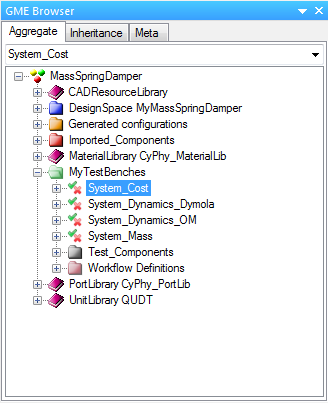
We will need to create an empty Parametric Exploration Model in order to proceed. To do this, right-click on MyTestBenches and select Insert Folder ‣ Parametric Exploration. Name this new folder PCC. Then right-click the PCC folder and select Insert Folder ‣ Parametric Exploration. Name this model MSD_Dymola (or MSD_OM if working with OpenModelica). The GME Browser will now look like this:

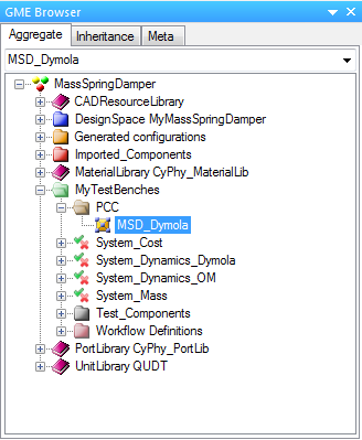
Open up the newly created parametric exploration model by double clicking on MSD_Dymola in the GME browser. This will open a new editing window.

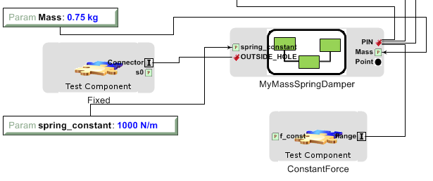
If you are using the model you created using the MSD Tutorial, you may need to add parameters for Mass and spring_constant to the System_Dynamics_Dymola (or System_Dynamics_OM if using OpenModelica) editing window. This may be accomplished by copy/pasting the “Mass” and “spring_constant” parameters from the “DesignSpace MyMassSpringDamper” -> “MyMassSpringDamper” folder in the GME Browser. If this is done, the window will appear as follows:

Step 1: Inserting the Test Bench Model

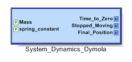
Copy the test bench model under study from the GME Browser to the MSD_Dymola editing window. You can do this by right-clicking “System_Dynamics_Dymola” (or “System_Dynamics_OM” if using OpenModelica) in the GME Browser and selecting “Copy”. Then right-click in the editing window and use “Paste Special” -> “As Reference” to paste in a reference to the model. The editing window will now contain a reference, which appears as follows:

Step 2: Inserting a PCCDriver

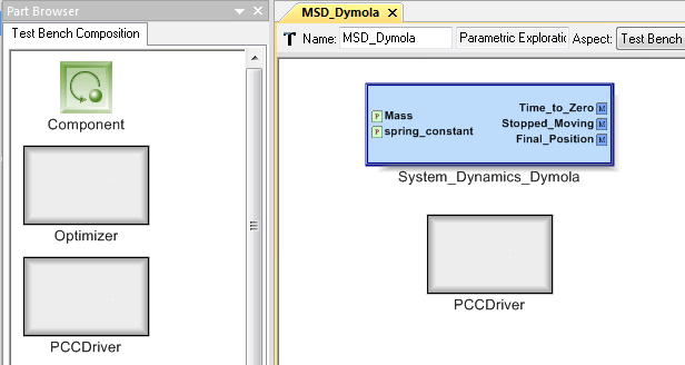
From the Part Browser, drag a PCCDriver object into the editing window:

Step 3: Adding parameter objects

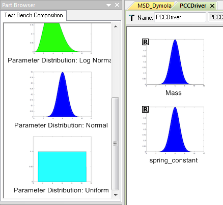
Open the new PCCDriver object by double-clicking on it. The PCCDriver now needs parameters added to match each parameter in the test bench model under study – in this case, the parameters “Mass” and “spring_constant”. Each parameter also needs a distribution. For this tutorial, we assume that the parameters are normally distributed. Drag two icons for the normal distribution from the Part Browser to the editing window, and rename them “Mass” and “spring_constant”, as follows:

Any object can be renamed easily using the Object Inspector. The four available parameter types each represent a different random variable distribution, each defined by distribution-specific parameters:

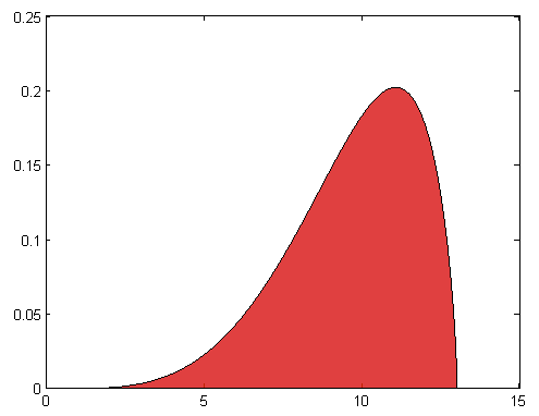
The Beta Distribution: Unlike the normal distribution, the Beta distribution has finite upper and lower bounds (defined by upper and lower limits) and can be symmetric or non-symmetric (defined by two shape parameters).

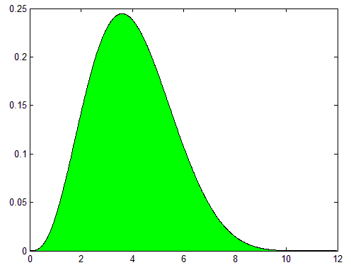
The Log-Normal Distribution: defined by a shape and a log scale parameter. The log-normal distribution is similar to the normal distribution but has a lower limit of 0 instead of –infinity.

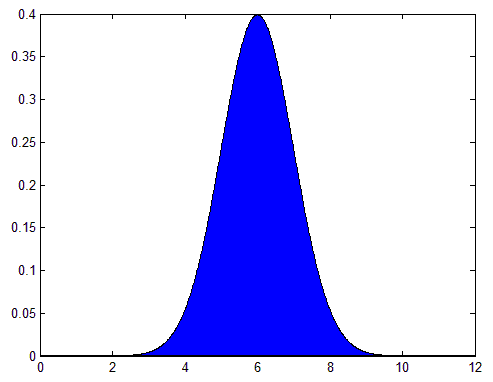
The Normal Distribution: defined by its mean and standard deviation. The normal distribution is always symmetric and is defined over the range [-infinity, infinity] .

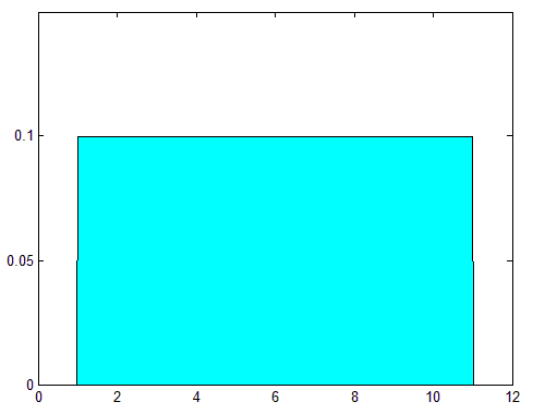
The Uniform Distribution: defined by its upper and lower limits. Every outcome between the limits is equally probable.

Step 4: Setting the distribution-specific parameters for each parameter

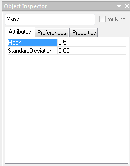
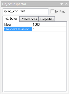
To do this, select a parameter in the editing window, then modify the parameter fields in the Attributes tab of the Object Inspector. We will set the mean of the Mass parameter to “.5” and the standard deviation to “.05”. Likewise, we’ll set the mean of the spring_constant parameter to “1000” and the standard dev iation to “50”, as shown below:

Step 5: Adding PCCOutput objects

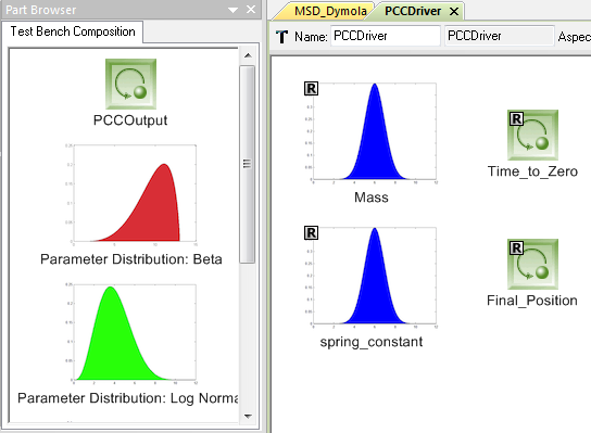
Drag a PCCOutput object from the Part Browser to the editing window for each output of the test bench model it is desired to measure, and rename them appropriately. In this case, we are interested in the two continuous outputs, “Time_to_Zero” and “Final_Position”:

Step 6: Configuring the PCCOutput objects

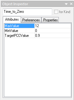
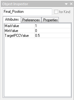
Per design specifications, each model output variable has an acceptable range, i.e. a range of values an output may take and be considered a successful simulation. After selecting a PCCOutput object, its acceptable range must be set by modifying the MaxValue and MinValue fields in the Attributes tab of the Object Inspector. The simulator will later calculate a PCC value for this range of outputs, which captures the probability that the output will remain in the specified ranges given the input distributions. The TargetPCCValue specifies the minimum probability that this calculated PCC value will fall between its MaxValue and MinValue values and still be considered a successful configuration.

For this tutorial, set the Min and Max values of Time_to_Zero to 0 and 12 respectively, with a TargetPCCValue of 0.9. This specifies that we desire a 90% probability that the mass in our MSD model will reach 0 velocity within 12 seconds. Likewise, set the Min and Max values of Final_Position to 0 and 1 respectively, with a 0.5 TargetPCCValue. This specifies that we desire at least a 50% probability that the final position of the mass will lie between 0 and 1:

Step 7: Selecting the Uncertainty Propagation (UP) and Sensitivity Analysis (SA) Methods

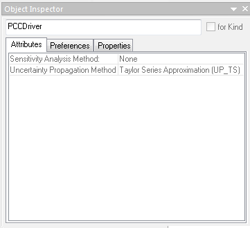
After selecting the PCCDriver object by clicking on it in the MSD_Dymola editor window, we can select the UP_Method and/or SA_Method we wish to use via drop-down menus in the Attributes tab of the Object Inspector. We will be using the default option of a Taylor Series approximation for this tutorial, as it is very fast to calculate and requires only 5 simulations given the two inputs we are using:

Each of the available methods differs in the way it samples from the space defined by the parameter distributions:

UP Methods

Monte Carlo Simulation (MCS): Random samples eventually cover the entire space. This is the most robust method, but requires thousands, or even millions, of samples to provide an accurate representation of the output distribution. Prov ides an approximation of the entire output distribution space.

Taylor Series (TS) Approximation: Also known as the Mean Value First Order Second Moment (MVFOSM), this method performs a first-order Taylor expansion very near the mean values of all parameters. The fastest method. Accurate only for linear or nearly linear problems. Provides a Normally distributed approximation of the entire output distribution space.

Most Probable Point (MPP) Method: Also known as the Hasofer and Lind (HL) First Order Reliability Method (FORM), this method searches the parametric space iteratively, looking for the most probable point of failure. The method then performs a first-order Taylor expansion around that point. Provides only the probabilities of being between the limits.

Full Factorial Numerical Integration (FFNI): Applies the Gaussian quadrature numerical integration technique. Sampling is done only at the quadrature nodes. Pro ides an approximation of the entire output distribution space.

Univariate Dimension Reduction (UDR) Method: Like the FFNI method, but ignoring interaction effects between the parameters. Almost as fast as TS, yet much more accurate. Provides an approximation of the entire output distribution space.

Polynomial Chaos Expansion (PCE): A polynomial expression in terms of standard normal variables is fitted as a surrogate model. An MCS is then applied to the surrogate, which is very fast to evaluate. Provides an approximation of the entire output distribution space.

For more information on the various uncertainty propogation methods, please consult the paper “System-level Design Reliability Enabled by Copulas”, by Christopher Hoyle and Irem Tumer.

SA Methods

The Sobol method, also known as the (Quasi) Monte Carlo method, uses the first order sensitivity index by decomposing the model function into summands of increasing dimensionality. The approach has been expanded by subsequent researchers to include computation of the total sensitivity index. The integrals utilized in the analysis can be computed with Monte Carlo methods.

The main idea underlying the Fourier amplitude sensitivity testing (FAST) method is to convert the k-dimensional integral into a one dimensional integral. Each uncertain input factor is related to a frequency ω and transformed by X(s) = Gi(sin(ωs)), where Gi is a suitably defined parametric equation which allows each factor to be varied in its range, as the parameter s is varied. The set {ω1,…, ωk} are linearly independent integer frequencies. FAST only provides the first-order indices.

In 1999, researchers proposed an improvement of the FAST method. They called it the Extended Fourier Amplitude Sensitivity Test (EFAST). With this method they could estimate the total effect indices, as in the Sobol method, by estimating the variance in the complementary set. This is done by assigning a frequency ω for the factor X (usually high) and almost identical frequencies to the rest ωi (usually low). Step 8: Connecting the Test Bench Model to the PCCDriver

By this point, the parametric exploration model should have two components, a reference to the Test Bench Model, and the PCCDriver. Using the Connect Mode, connect each of the parameters on the PCCDriver to the corresponding parameter on the reference to the test bench model. Then connect each of the outputs from the reference to the Test Bench Model to the corresponding outputs on the PCCDriver, as follows:

The “PCCDriver” object can be widened by setting “Preferences” -> “PortLabel Length” to “0” in the Object Inspector.

Step 8: Connecting the Test Bench Model to the PCCDriver

By this point, the parametric exploration model should have two components, a reference to the Test Bench Model, and the PCCDriver. Using the Connect Mode, connect each of the parameters on the PCCDriver to the corresponding parameter on the reference to the test bench model. Then connect each of the outputs from the reference to the Test Bench Model to the corresponding outputs on the PCCDriver, as follows:

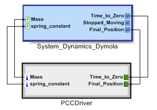
The “PCCDriver” object can be widened by setting “Preferences” -> “PortLabel Length” to “0” in the Object Inspector.

Step 9: Running the Simulations

Click the CyPhy Master Interpreter button () in the toolbar. Select the configurations to run, then click OK.

Step 10: Interpreting the results

There are two ways the PCC text output can be accessed once the simulation is finished. One way is to right-click the job in the JobManager when it is finished and select “Show in explorer”. The second is to click on the link provided in the GME Console after the words “Generated files are here:”.

Once you have entered the PCC directory, you will see several files that were used to either run the simulation, or were output from the simulation. The two files of interest to us now are “stdout.txt” and “testbench_manifest.json”. If we open the former and scroll to the bottom, we will see an output like this:

Correlation:
[[ 1.  1.]
 [ 1.  1.]]
Moments:
  Mean = [ 1.          6.80000019]
  Variance = [ 0.00250014  0.99999809]
  Skewness = [[ 0.]
 [ 0.]]
  Kurtosis = [[ 3.]
 [ 3.]]
PCC: [0.5, 0.99999990035306252, 0.5]
Complexity estimates: [0.2038907047155587, 4.1327274127362008]
Done!
Elapsed time:  25.0759999752 seconds

These are some of the statistical data generated from the PCC run. We can see a correlation matrix, moments of the output distributions, and the PCC calculated for each of the outputs. The PCC values displayed here show that there is a 50% chance that the limits of the first output (in this case, “Final_Position”) will be met, and nearly a 100% chance that the limits of Time_to_Zero will be met. Together, these produce a probability of 50% that ALL limits will be met, which is the final value shown in the PCC vector. It is these PCC values that are tested against the “TargetPCCValues” of the various PCCOutputs discussed above. A complexity estimate for the output distributions is also provided.

The second file of use is “testbench_manifest.json”. This file contains a summary of all the inputs and outputs of the simulation. Covariance and correlation matrices are available here, as well as the moments, PCC values, and complexities of the various output distributions.