Advanced Topics
Common Workflows
Using a Test Bench to Extract Properties
Often various Property and Parameter values from Components or Component Assemblies in the OpenMETA project are needed in the context of a PET to drive the parameters of the various Analysis Blocks; the best way to get these values is to use a Test Bench.
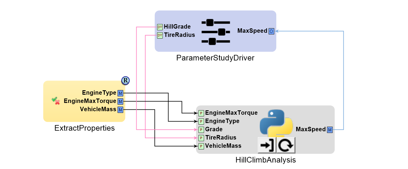
PET with a Test Bench to extract Properties from the OpenMETA Project
See the Common Utilities section of the Test Bench chapter for information on how to do this.
Optimization
Hot Start vs. Cold Start
It is fairly common to have an Optimizer PET Driver that runs repeatedly as part of a larger Design of Experiments (e.g. see PET Nesting).
In these situations the user can choose between “Hot Start” and “Cold Start.”
What is “Hot Start?”
In “Hot Start,” each time the nested Optimizer PET is called by the higher-level Parameter Study PET, it starts the optimization process using the final Design Variable values that it solved for during the last Parameter Study iteration.
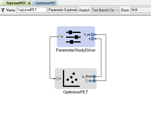
The TopLevel PET contains a Parameter Study Driver and a nested OptimizerPET
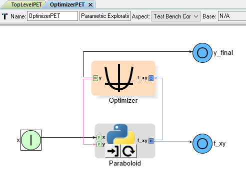
The OptimizerPET contains an Optimizer Driver and a Python Wrapper Component
In the “Hot Start” example above, for the first iteration of the TopLevel PET’s Parameter Study Driver, the Optimizer PET starts the optimization process using the Design Variable y’s initial value of 0.0; however, for each subsequent iteration of the top-level Parameter Study Driver, the lower-level Optimizer Driver uses the previous iteration’s final value of y as its starting point.
For many cases, “Hot Start” is faster and more efficient. Because the top-level Parameter Study Driver generally changes its Design Variables in an incremental fashion, the lower-level Optimizer Driver’s previous solution is usually much closer to the new solution vs. whatever its initial Design Variable values were.
“Hot Start” is the default behavior for the Optimizer PET Driver’s COBYLA optimization method.
What is “Cold Start?”
In “Cold Start,” each time the nested Optimizer PET is called by the higher-level Parameter Study PET, it starts the optimization process using the same initial Design Variable values.
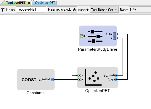
The TopLevel PET contains a Parameter Study Driver, a Constants block, and a nested OptimizerPET
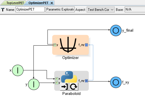
The OptimizerPET contains an Optimizer Driver and a Python Wrapper Component
In the “Cold Start” example above, the lower-level Optimizer Driver’s Design Variable y is connected directly to the Problem Input y, which is being driven from the Constants block in the top-level PET.
As a result, for every iteration of TopLevel PET’s Parameter Study Driver, the Optimizer PET starts its optimization process using the same starting point for its Design Variable y.
The advantage of “Cold Start” is that it prevents individual optimizations from interfering with one another. Occasionally, with the Optimizer Driver’s COBYLA method, an optimizer run can diverge, causing the Design Variable values to violate their range constraints. In a “Hot Start” setup, one divergence will likely “ruin” all subsequent Optimizer Driver runs, but in a “Cold Start” setup, the forced restart limits the impact of outliers on the entire set of results.
Setting Initial Conditions
Occasionally, an optimization problem’s objective function will feature numerous local minima (or maxima), making it harder to find a global minimum using just an Optimizer Driver.
In these situations, it may be useful to nest a PET with an Optimizer Driver inside another PET with a Parameter Study Driver as shown below.
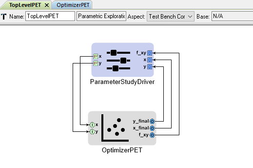
The TopLevel PET contains a Parameter Study Driver and a nested OptimizerPET
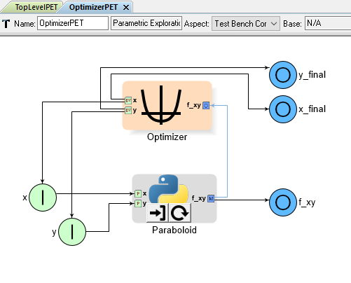
The OptimizerPET contains an Optimizer Driver and a Python Wrapper Component
The Parameter Study Driver in the top-level PET varies the initial values of x and y. These are then passed into the lower-level PET to provide the Optimizer PET with different starting points each time. This strategy increases the chances of finding the global minima.
Adding Design Variable Constraints
A constrained optimization problem is one where an Objective is being minimized with respect to Design Variables that are restricted to a specific range.
For example, one might wish to minimize a car’s fuel consumption per mile with respect to tire radius while requiring that the tire radius remain between 13” and 17”.
OpenMETA supports constrained optimization via the Optimizer PET Driver’s COBYLA Function (COBYLA = Constrained Optimization BY Linear Approximation); however, the user must manually connect each Design Variable to a matching Optimizer Constraint and set the Optimizer Constraint’s MinValue and(or) MaxValue to the Design Variable’s desired minimum and maximum values.
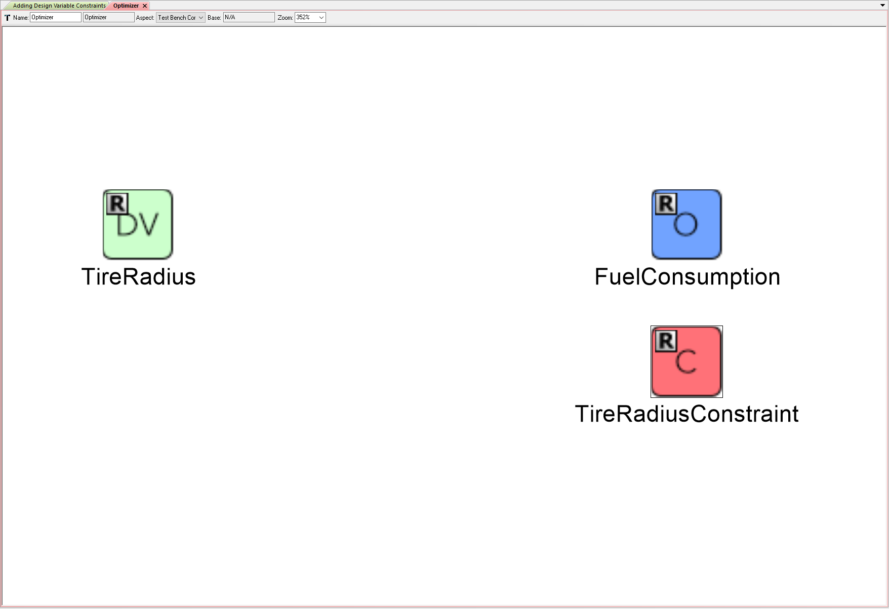

TireRadius’s desired range entered into corresponding Optimizer Constraint’s Attributes
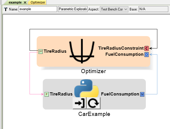
TireRadius Design Variable connected directly to corresponding Optimizer Constraint
In contrast, no such workaround is needed if the Parameter Study PET Driver is being used)
Checking Optimization Results
The Optimizer PET Driver is a powerful tool but it cannot be used blindly.
Some functions (in particular non-convex functions) are quite difficult to optimize, and the Optimizer may not be able to reliably locate the global minimum.
The Optimizer PET Driver may:
- fail to converge within the maximum number of iterations.
- locate a local minimum and not the global minimum.
- violate Optimizer Constraints in order to converge.
The user must make sure that the final answer provided by the Optimizer does not significantly violate any of the Objective Constraints and that the Optimizer converged before executing the maximum number of iterations.
If the function contains numerous minima/maxima, the user might consider exploring the design space with another PET Driver (such as the Parameter Study) or setting up a multi-start Optimization problem by nesting the Optimizer PET inside a higher-level PET with a Parameter Study Driver providing different initial values to the Optimizer PET’s Design Variables.
Scaling/Normalizing Design Variables
The Optimizer PET Driver may struggle to converge if it contains Design Variables with ranges that differ by several orders of magnitude.
For example, one might wish to optimize a car’s fuel consumption per mile with respect to tire radius and weight, where tire radius can vary from 13” to 17” and weight can vary from 3200 lbs. to 4200 lbs. The range of the weight Design Variable is more than two orders of magnitude greater than the range of the tire radius Design Variable. Since the difference in magnitudes between the two Design Variable is so great, the Optimizer may struggle to successfully converge in this case.
Therefore, it is generally good practice to rescale or normalize Design Variables with ranges that differ by several orders of magnitude (or more).
For example, in the car problem above, the user could rescale the tire radius Design Variable (and associated Optimizer Constraint - this is a constrained optimization problem!) to vary from 130 to 170 units and the weight Design Variable (and associated Optimizer Constraint!) to vary from 320 to 420 units. The user could then insert PythonWrapper components to undo the scaling between the Design Variables and the CarExample PythonWrapper.
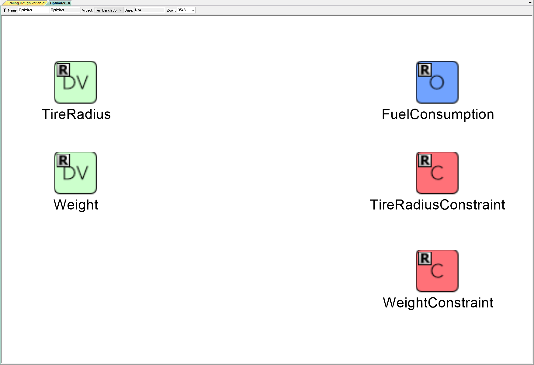

Scaled TireRadius Design Variable

Scaled Weight Design Variable

Scaled TireRadius Constraint

Scaled Weight Constraint
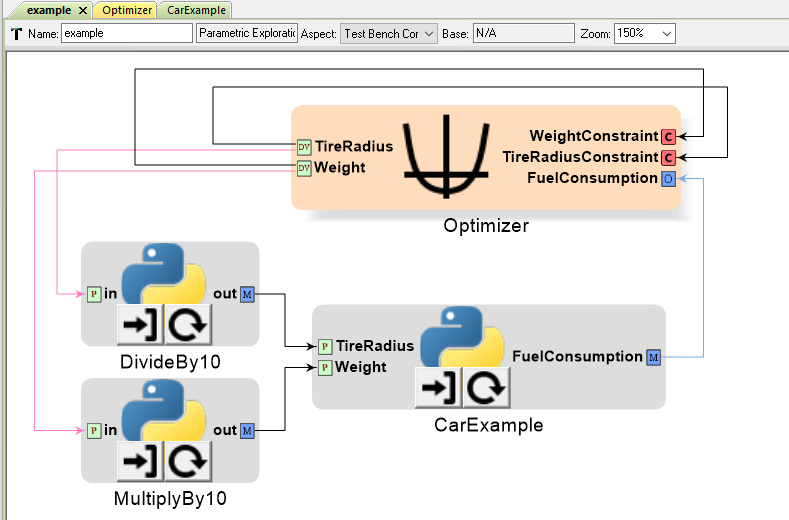
Undoing scaling for system analysis
Note
You would have to generate DivideBy10 and MultiplyBy10 blocks yourself. See the Python Wrappers section for details on creating your own Python Wrapper blocks.
Optimizing Non-convex Functions
Note
This section is under construction. Please check back later for updates!