Custom Tabs¶

The Visualizer framework is extensible, allowing one or more user-defined tabs to be rendered in a given instance of the Visualizer. The Visualizer is built using the statistical programming language R and a package called Shiny. When an instance of the Visualizer is launched, it consumes a config file that specifies both the data and the references to the desired tabs for that instance. Each tab is in turn implementeded as a single Shiny module in a .R file that includes the definition of both the UI and the backend functionality of a tab.

Basic Tab Structure¶

The basic structure of a custom tab is very simple. It must have the following variable and function definitions present to be valid:

title: This variable should be the desired title of the tab in the UI as a string.
footer: This variable should specify whether or not you want the Visualizer framework footer to be visible when this tab is opened. It will either be TRUE or FASLE.
ui(id): This function should have only the id parameter and return the output of a Shiny UI function, e.g. fluidPage(), that defines the desired UI.
server(input, output, session, data): This function is passed the following parameters:
- input: This is the Shiny ‘input’ list. You will use this to access inputs generated in the UI.
- output: This is the Shiny ‘output’ list. You will use this to assign values to outputs referenced in the UI.
- session: This is the Shiny ‘session’ object. It is used to access the ‘ns’ function and is consumed by some of the advanced Shiny functions.
- data: This data frame includes the raw data that was passed to the Visualizer by the Results Browser as well as a host of other relevant metadata about the dataset. See below for more infomation.

The ‘data’ Object¶

Upon launch, the Visualizer Framework builds an R data frame that includes the raw data and other useful metadata. The visualizer manages this data frame for the most part, and each of the custom tabs should only enjoy limited write-access to it.

The data object contains all the information that a tab needs to interact with the data and any of the other features that are provided by the Visualizer framework. Below is a mapping of the data structure with an explanation for each of the objects.

data - contains all the passed objects
- Colored - the filtered data that has an added ‘color’ column
- Filtered - the raw data that has been filtered by the different UI elements in the “Filters” section
- Filters - the state of each of the sliders, selectInputs, etc. in the “Filters” section of the Visualizer UI
  - <variable names>
    - type - the “R” data-type of the variable, e.g. ‘factor,’ ‘integer,’ or ‘numeric’
    - selection - (if type is ‘factor’), list of all selected choices
    - min, max - (if type is ‘integer’ or ‘numeric’)
- meta
  - coloring
    - <coloring names>
      - name - name of the coloring scheme
      - type - ‘Max/Min’ or ‘Discrete’
      - var - the name of the variable that is the basis of the coloring
      - goal - (for ‘Max/Min’) ‘Maximize’ or ‘Minimize’
      - palette - (for ‘Discrete’) ‘Rainbow,’ ‘Heat,’ ‘Terrain,’ ‘Topo,’ or ‘Cm’
      - rainbow_s - (if ‘Rainbow’ for palette) the saturation for the palette
      - rainbow_v - (if ‘Rainbow’ for palette) the value/brightness for the palette
    - current
      - name - name of the coloring scheme
      - type - ‘Max/Min’ or ‘Discrete’
      - var - the name of the variable that is the basis of the coloring
      - goal - (if type is ‘Max/Min’) ‘Maximize’ or ‘Minimize’
      - colors - (if type is ‘Discrete’, list) the list of the colors used for each variable
  - comments [Not yet implemented]
    - <comment ids>
      - id - a guid associated with the comment
      - username - the username of the user who wrote the comment
      - date - the date the comment was added
      - text - a guid associated with the comment
      - object - (optional) the object(s) referenced in the comment
  - pet - contains information about the PET that generated these results
    - sampling_method - (string) ‘Full Factorial,’ ‘Central Composite,’ ‘Opt Latin Hypercube’, or ‘Uniform’
    - num_samples - (integer) the ‘num_samples’ value from the ‘code’ field in the OpenMETA project
    - pet_name - (string) the name of the ‘Parametric Exploration’ in the OpenMETA project
    - mga_name - (string) the name of the .mga file within which the PET resides
    - generated_configuration_model - (string) the name of the ‘Generated Configuration Model’ created by the DESERT tool that was selected for the execution of this PET
    - selected_configurations - (list) the names of each of the configurations that were chosen for this PET execution
    - design_variable_names - (list) the names of all variables that were of type ‘Design Variable’
    - design_variables - (list) detailed information about the variables that were of type ‘Design Variable’
    - objective_names - (list) the names of all variables that were of type ‘Objective’
    - pet_config - (data frame) the parsed pet_config.json file.
    - pet_config_filename - (string) the filename of the ‘pet_config.json’ file relative to the location of the ‘visualizer_config.json’ file.
  - sets [Not yet implemented]
    - <set names>
      - name - name of the set
      - username - the username of the user who created the set
      - date - the date the set was added
      - objects - the different objects in the set, most often design configurations
  - variables
    - <variable names>
      - name - corresponds to variable in data$raw df
      - name_with_units - unit appended in parentheses
      - type - ‘Unknown’, ‘Design Variable’, ‘Objective’, or ‘Classification’
      - username - the username of the user who wrote the comment
      - date - the date the comment was added
- pre - basic preprocessing reactives to simplify interaction with the data
  - var_names() - (list) original names of all the variables in the input data set
  - var_class() - (list) the class (or type) of each of the variables
  - var_facs() - (list) names of all the variables of class ‘factor’
  - var_ints() - (list) names of all the variables of class ‘integer’
  - var_nums() - (list) names of all the variables of class ‘numeric’
  - var_nums_and_ints() - (list) names of all the variables of class ‘numeric’ or ‘integer’
  - abs_max(), abs_min() - (list) the maximum and minimum values for each variable in var_nums_and_ints
  - var_range_nums_and_ints() - (list) names of all the variables of class ‘numeric’ or integer’ that vary across some range, i.e. are not constants
  - var_range_facs() - (list) names of all the variables of class ‘factor’ that vary across some range, i.e. are not constants
  - var_range() - (list) names of all variables that vary across some range, i.e. are not constants
  - var_range_nums_and_ints_list() - (list of lists) var_range_nums_and_ints() sorted into lists by type
  - var_range_facs_list() - (list of lists) var_range_facs() sorted into lists by type
  - var_range_list() - (list of lists) var_range() sorted into lists by type
  - var_constants() - (list) names of the variables of any class that don’t vary in the dataset
- raw$df - the raw data with no filtering or coloring applied as a reactive value

E.g. In your server function, you could find the type of the first variable by evaluating data$meta$variables[[1]]$type in either a reactive context or within an isolate() call. You could also find a list of all the variables that are factors, i.e. discrete choices, in the data$raw$df data frame by evaluating data$pre$var_facs()

Histogram Example Tab¶

Below is an example tab definition .R file.

title <- "Histogram"
footer <- TRUE

ui <- function(id) {
 ns <- NS(id)

 fluidPage(
   br(),
    column(3,
     selectInput(ns("variable"), "Histogram Variable:", c())
   ),
   column(9,
     plotOutput(ns("plot"))
   )
 )

}

server <- function(input, output, session, data) {
 ns <- session$ns

 observe({
   selected <- isolate(input$variable)
   if(is.null(selected) || selected == "") {
     selected <- data$pre$var_range_nums_and_ints()[1]
   }
   saved <- si_read(ns("variable"))
   if (is.empty(saved)) {
     si_clear(ns("variable"))
   } else if (saved %in% c(data$pre$var_range_nums_and_ints(), "")) {
     selected <- si(ns("variable"), NULL)
   }
   updateSelectInput(session,
                     "variable",
                     choices = data$pre$var_range_nums_and_ints_list(),
                     selected = selected)
 })

 output$plot <- renderPlot({
   req(input$variable)
   hist(data$Filtered()[[input$variable]],
        main = paste("Histogram of" , paste(input$variable)),
        xlab = paste(input$variable))
 })

}

The title of the tab is assigned on line 1. On line 2 we specify that we want to display the Visualizer footer when this tab is open.

The UI for this example tab, defined in ui(id) on lines 4-17, is simply a select box for the user to choose which variable to process for the histogram and a placeholder for the histogram plot itself; the select box inputId and plot outputId are ‘variable’ and ‘plot’, respectively. The Visualizer framework implements the Shiny ‘Module’ concept to isolate the tabs and avoid input name collisions; this necessitates the ns <- NS(id) statement at the beginning of the function and the wrapping of all the inputId and outputId parameters to Shiny UI function calls in a call to ns().

The server function, defined on lines 19-45, is where we describe the backend processing that produces plots and other outputs for the UI.

The body of this function begins by assigning the local namespace function (session$ns) to ns on line 20. Although you do not need to call ns() when accessing variables from input, e.g. the input$variable reference on line 42, you do need to wrap inputIds and outputIds as we did in the UI definition above when they are being created or updated.

It then implements an observe() call on lines 22-36 to properly update the options presented to the user in the “Histogram Variable” select box. In Shiny, an observe() provides a mechanism for re-running a block of code when any of the reactive variables referenced within that code are initialized or changed. In this case we want to update the choices presented in the ‘variable’ Select Input anytime the non-constant, numeric or integer variables in our dataset change. (This occurs when the data is initialized or classifications are added or removed.)

This code block is fairly complex, but it provides a lot of functionality: it specifies a default value, loads a value saved from a previous session, and updates the ‘variable’ UI element dynamically as the dataset is altered. The selected variable is first assigned the current value of the input. This is done within an isolate() call which breaks the reactive dependency on the input value; without the isolate() our code block would be executed every time the user changed the input. Next we assign a default value if it is currently null or empty, .e.g. when the Visualizer is launched for the first time. Then we use the si_read() function to check if there is a saved value for this input from a previous session of the visualizer. (Note the use of the ns() call around our input name.) The is.empty() function is a custom function that evaluates to true if the value is either null or an empty list(). To cover the case of it being an empty list, we clear the saved value as it would prevent saving the value of this input upon closing the current session. The final if statement ensures that the saved choice is in the currently available options before applying the value. Lastly we call updateSelectInput to update the input with our new values.

The final section of code on lines 38-43 defines the ‘plot’ output to be a histogram of the variable selected in the “Histogram Variable” select box with a title and x-axis label. The req() function allows us to break if a needed input is NULL as is the case with input$variable before the dataset is initialized and all the reactive dependencies are sorted out.

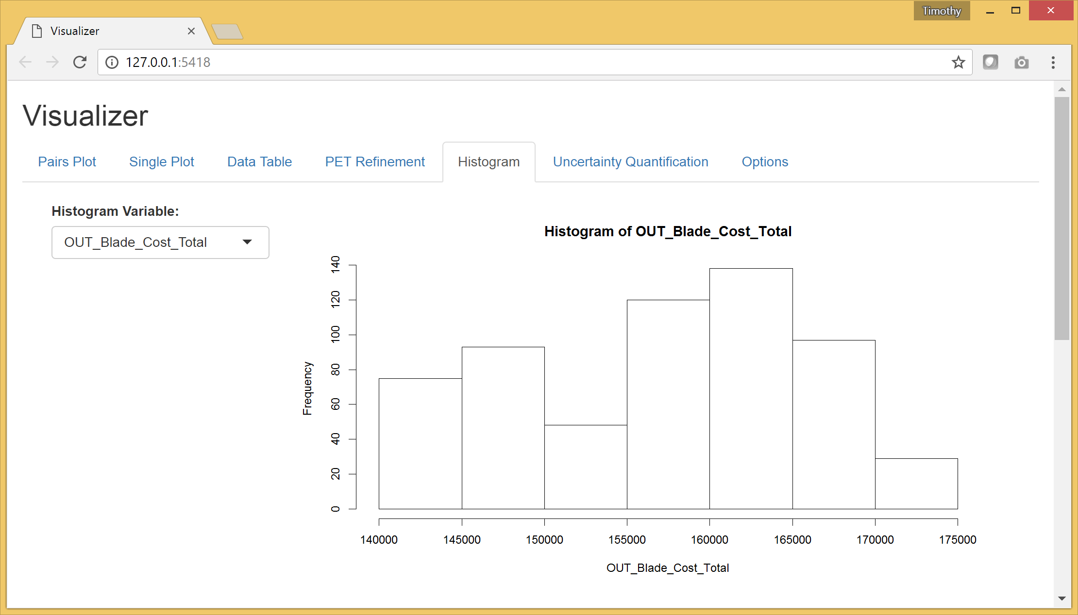
The rendered tab looks like this:

This example can be found at C:\Program Files (x86)\META\bin\Dig\tabs\Histogram.R (or wherever you installed OpenMETA) and used as the basis for creating tabs of your own.

Adding Your Own Tab¶

Creating the File¶

Navigate to C:\Program Files (x86)\META\bin\Dig\tabs\ to see all the currently-configured user-defined tabs. Each file here corresponds to a single tab in the Visualizer. To create a tab of your own, simply make a copy of the Histogram.R (or other) file and modify it to suit your needs. The next time you launch the Visualizer, your tab will be included in the tabset.

Note

The tabs are added in the order that they appear in this directory, so it may be useful to prepend a number to the filename.

Developing your Application¶

We recommend using RStudio to develop your custom tabs. It offers syntax highlighting, code completion, and debugging support. After downloading and installing the software, you should be able to open the Dig.Rprog project file at C:\Program Files (x86)\META\bin\Dig\ and launch the Visualizer directly from RStudio.

To enable breakpoints in RStudio in your tab file code you will have to comment (Control-Shift-C) the debug call and uncomment the debugSource calls towards the top of server.R file.

# Source tab files
print("Sourcing Tabs:")
tab_environments <- mapply(function(file_name, id) {
   env <- new.env()
   if(!is.null(visualizer_config$tab_data)) {
     env$tab_data <- visualizer_config$tab_data[[id]]
   } else {
     env$tab_data <- NULL
   }
   # source(file_name, local = env)
   debugSource(file_name, local = env)
   print(paste0(env$title, " (", file_name, ")"))
   env
 },
 file_name=tab_files,
 id=tab_ids,
 SIMPLIFY = FALSE
)

In some cases you may not experience proper breaking behaviour using standard breakpoints. You can place a browser() call in your code at the location you desire to break, and this should result in the execution pausing and an interactive prompt being shown when the call is reached.