This chapter presents several example projects that illustrate many of the capabilities of the META tools.

Android/Firmware Communication Example

This section presents an example of the Android/Firmware communication capability of the META tools.

With the production Ara platform, modules will communicate with apps via the UniPro bus built into the Endo. This example uses the SCBus bridge to emulate this communication between module and application, allowing you to prototype app/firmware interactions without having to build hardware or acquire an Ara Development Kit.

The Simulation Architecture Overview section describes how the SCBus bridge works. Running the Demonstration Model will show you how to get the sample application and firmware up and running on your own computer. The final section, A Detailed Look, will go into further detail on each element, and will help you use the simple example as a jumping-off point for your own designs.

Simulation Architecture Overview

The figure below shows a high-level overview of the example system being modeled. An Application Processor Module and a Peripheral Module communicate with each other via UniPro. In this example, Android software running on the Application Processor can communicate with firmware running on a microcontroller on the Peripheral Module.

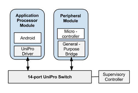
High-Level Overview of the Modeled ARA System

This High-Level Overview borrows from Figure 5.1 - Module to Module Communication (with Native UniPro Support and Bridge ASICs) on page 58 of the Project ARA Module Developer Kit (MDK) Release 0.11. The test environment used to model this ARA system is shown in the following figure.

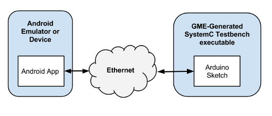
High-Level Overview of the Test Environment

Compare this figure to the previous one. On the left is an Android emulator or a cell phone, corresponding to an ARA AP module. The emulator/cell phone runs an Android app corresponding to the one running on the AP module. On the right is a SystemC hardware behavioral simulation, representing an ARA peripheral module. The Arduino Sketch block corresponds to microcontroller firmware running on a microcontroller in the Peripheral Module.

Instead of UniPro, this test environment uses User Datagram Protocol (UDP) packets sent over a wired or wireless Ethernet network to link the emulator/cell phone and the SystemC hardware behavioral simulation. Alternatively, if both an Android emulator process and a SystemC test process are running on the same PC, the network can be internal to the PC.

The Android app in the test environment is a regular Android app, except it also imports the SCBus (SystemC Bus) package that allows it to communicate with the SystemC test process over UDP.

The SystemC hardware behavioral simulation communicates with the Android app as follows: The SystemC test process includes a simulated ATmega microprocessor, which runs user-supplied Arduino Sketch (.ino) firmware. The firmware uses the simulated ATmega's UART to communicate with the Android app. The SCBus function within the simulation handles the mapping between the simulated UART's data and the UDP-based SCBus protocol.

Resources

The example META project for this feature can be found on the Downloads page. The modeling project includes two .xme files.

Meta Project Filename	Description
`Simple_SystemC_model.xme`	A simple design featuring only a microcontroller on which to run the example firmware.
`SAMI_SystemC_model.xme`	Based on the Ara Prototype Module, this includes a microcontroller which runs the example firmware.

The example Android app for this feature is included with the META tools install.

Android App Project Path	Description
`C:/Users/Public/Documents/META Documents/SystemC_Android/SystemCTest`	A simple Android app that uses the communication bridge discussed in this demo

Running the Demonstration Model

Running the demonstration involves three main parts:

Generating the SystemC-based simulation from the CyPhy model.
Compiling and running the example Android app.
Interacting with the app and observing the results.

Opening the Model and Generating the Hardware Simulation

After downloading the modeling project described in the Resources section above, unzip it to a directory. Open Simple_SystemC_model.xme to load the project.

To generate the simulation, open the SystemCBehavior test bench, found at path /Testing/SystemCBehavior. Execute the test bench by running the Master Interpreter. Be sure that Post to META Job Manager is selected.

Once the new job completes in the Job Manger, open the results folder by clicking the link that reads "Generated files are here", as shown below:

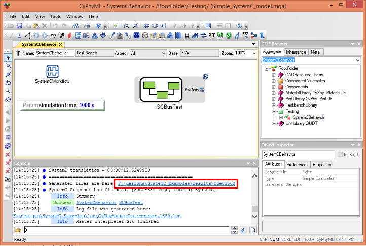
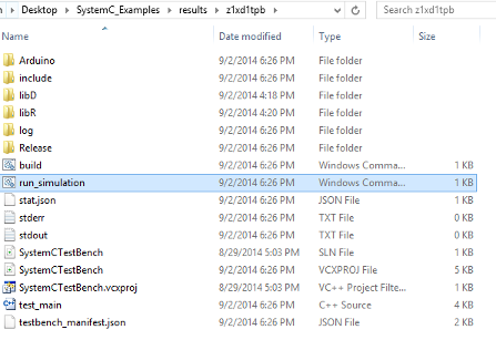
The results folder will contain a number of artifacts, including a file named run_simulation.cmd. This is the command that we'll run later to execute the hardware simulation, but we'll wait until we get the Android app up and running.

Opening and Running the Android App

The example Android application is included with the META tools install, and its location is described in the Resources section above. Currently, the example application is only configured to compile using the Eclipse ADK. Support for Android Studio is in the works.

Compile the SystemCTest project and run it in an emulator. Once the app has loaded, you're ready to start running the Hardware Simulation.

Note: The details of compiling Android apps varies by the environment, and isn't covered here. For more information, check the documentation that comes with your Android development environment.

Running the Hardware Simulation

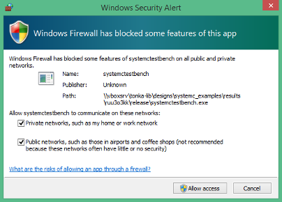
Now build and execute the hardware simulation by running run_simulation.cmd from the results folder. When prompted, choose to allow the simulation to communicate on both Public and Private networks:

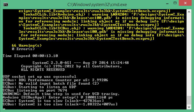
Once the compilation is finished, the window will begin to display status messages, as shown below. Now, we can begin interacting with the simulation using the Android app.

Interacting With the Simulation

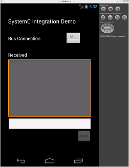
Click the app's Bus Connection button, so that its state switches to "On". Enter numbers or text into the white text box near the bottom. Click Send to transmit the data to the hardware simulation.

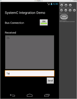
The data sent by the app is read by the simulated microcontroller firmware by reading from a virtual serial port. The firmware takes each character of input and increments it by one. Thus, "1" will become "2", and "a" becomes "b". Once the microcontroller firmware has processed the input, the result is sent back via the virtual serial port, is received by the Android app, and finally is displayed in the large grey text box.

A Detailed Look

This section goes into detail about the firmware and Android code used for this example.

Microcontroller Firmware

The microcontroller simulation model loads and executes user-provided firmware as part of its execution. This subsection will discuss the how the runtime firmware's location is specified, what syntax is supported, and what the example program does.

How the Runtime Firmware's Location is Specified

The runtime firmware of the demonstration model is in an Arduino sketch (.ino) file named SCBusApp.ino. The path to this file is specified via a property reference named Source, within the ATMEGA48_SCBussApp component model (shown near the top right of the figure below).

The path to the SCBusApp.ino file in the Source property is relative to the project's root directory. To run different firmware in the simulation, this is the property to change.

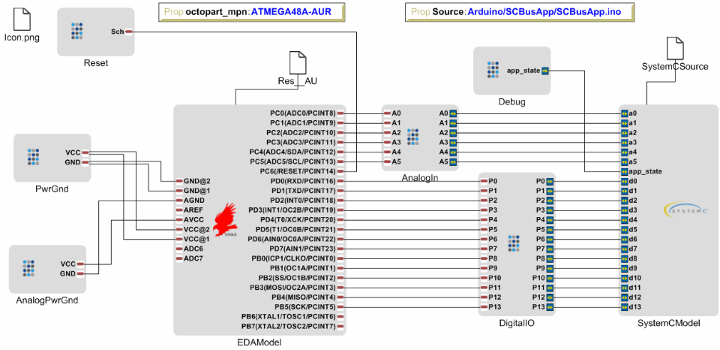
ATMEGA48_SCBussApp component model

Connecting All Analog Inputs

Also seen in the right of the ATMEGA48_SCBussApp component model is the SystemCModel. The SystemCModel has cerulean-colored SystemCPorts, representing the inputs and outputs of the SystemC ATmega model. For the demo, most of these ports aren't used and need not be externally connected. The exceptions are ports a0-a5, the analog input ports. SystemC requires that all input ports be driven; otherwise, generating the SystemC executable will fail. To prevent this, the analog inputs are connected to a SystemC analog ground component in the Component Assembly where the ATMEGA48_SCBussApp component is instantiated, as shown in the figure below.

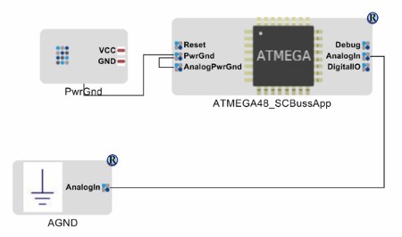
SCBusTest Component Assembly

Supported Firmware Syntax

Arduino sketch firmware is described in the Language Reference of the Arduino website. At present, only a subset of the Arduino sketch language features are supported in the SystemC model. Specifically, importing libraries is not supported. In general, syntax that is part of the C programming language is supported, including control structures, comments, and operators.

Supported Arduino-specific constants include HIGH, LOW, INPUT, OUTPUT, and INPUT_PULLUP.

Supported Arduino Sketch functions:

void pinMode(int pin, int mode);
void digitalWrite(int pin, int val);
int digitalRead(int pin);
int analogRead(int pin);
void analogWrite(int pin, int val);
unsigned long millis();
unsigned long micros();
void delay(int ms);
void delayMicroseconds(unsigned int us);
int serial_read();
int serial_available();
void serial_write(int val);

NOTE: In the demo firmware, the serial communication functions read, write, and available are overridden, providing the interface between the firmware and the UDP-based scbus.

What the Example Firmware Program Does

The SCBusApp.ino firmware receives data bytes from the UART, increments them, and returns them over the UART. So, for instance, if an Android app sent the ASCII data bytes representing the characters "a", "b", and "c" to the SystemC test process via the scbus, the SCBusApp.ino firmware should receive those bytes, increment them, and return them, resulting in the Android app receiving the bytes "b", "c", and "d". The firmware also sets the duty cycle of a PWM output based on the value of the received byte. (On an Arduino, this would alter the brightness of an LED.)

The SCBusApp.ino firmware is reproduced below. It has an initial comment and some const int statements that can be mostly ignored. Then, like standard Arduino sketch firmware, it has setup() and loop() functions. The setup() function is called during initialization, and the loop() function is called afterward.

In this example, the setup() function initializes the simulated UART to 9600 bits per second, and the loop() function continually checks for a data byte from the UART. Once such a byte is available, the loop function:

Reads the byte,
Uses it to set the PWM duty cycle of the simulated ATmega's pin 13, and
Writes the received byte, incremented, back to the serial port.

// SCBus firmware example
const int analog0Pin = 22;
const int analog1Pin = 19;
const int pwm0Pin = 13;
const int pwm1Pin = 14;
const int pwm2Pin = 15;
const int ANALOG_MAX = 1023;
const int ANALOG_MIN = 0;
const int PWM_MAX = 255;
void setup() {
  Serial.begin(9600);
}
void loop() {
  if (Serial.available() > 0) {
    int inByte = Serial.read();
    // Use incoming value as PWM duty cycle
    analogWrite(pwm0Pin, inByte);
    // Send back some data
    Serial.write(inByte + 1);
  }
}

Although this sketch firmware doesn't need to know the network address of the app it communicates with, the simulated processor does need to know it. Currently the network address is coded in the processor component model as 127.0.0.1:2003, so it is expecting to connect to an Android emulator on the same PC.

Android Application Code

The Android application uses a library called SCBus to communicate with the simulated firmware. To use SCBus, one of the application's classes must implement the SCBusListener interface. If an instance of this class is passed into the open() method of an SCBus instance, then the dataReceived(byte[]) method of the listener will be invoked when data is received.

The Example Application

In the example below, the MainActivity of the app implements the SCBusListener interface. An instance of SCBus is stored as a member variable of this class, and it's initialized when the class is created.

The operation of the SCBus class can be turned on an off via the open(SCBusListener) and close() methods. In the example, this is toggled with the button marked BusConnection. When BusConnection is enabled, its handler, onBusButton() calls either the open() or close() method of the SCBus instance. The open(SCBusListener) method accepts the running instance of MainActivity, and when data is received from the microcontroller simulation, its dataReceived(byte[]) method is invoked. The callback function then writes that data to the text box.

package tonka.systemctest;
import tonka.scbus.SCBus;
import tonka.scbus.SCBusListener;
[...]
public class MainActivity extends Activity implements SCBusListener {
    private final String TAG = "SystemCTest";
    private SCBus bus;
    @Override
    protected void onCreate(Bundle savedInstanceState) {
        super.onCreate(savedInstanceState);
        setContentView(R.layout.activity_main);
        bus = new SCBus();
    }
    public void onBusButton(View view) {
        boolean on = ((ToggleButton) view).isChecked();
        if (on) {
            bus.open(this);
        } else {
            bus.close();
        }
        Button sendButton = (Button) findViewById(R.id.sendButton);
        sendButton.setEnabled(on);
    }
    public void onSendButton(View view) {
        EditText text = (EditText) findViewById(R.id.sendText);
        bus.send(text.getText().toString().getBytes());
        text.setText("");
    }
    protected void onDestroy() {
        Log.d(TAG, "onDestroy");
        bus.close();
        super.onDestroy();
    }
    [...]
    @Override
    public void dataReceived(byte[] data) {
        Log.d(TAG, "dataReceived :" + new String(data));
        EditText text = (EditText) findViewById(R.id.receivedText);
        text.append(new String(data));
    }
}

This concludes the discussion of the Android/Firmware communication example.

RF Analysis: 2.4 GHz Inverted-F Antenna

This section presents a case study of the RF Analysis capability of the META tools using a 2.4 GHz Inverted-F antenna example model. It shows the usage of the META RF models and testbenches.

The physical dimensions and the material properties of the generated RF model are based on the ARA prototype module templates described in the ARA MDK v0.11 reference materials.

Resources

The example model of the Ara module mounted Inverted-F antenna relies on the following files:

Filename	Description
InvertedF.xme	A META project that models the Ara prototype endo, module and the Inverted-F antenna.
InvertedF.xml	Geometrical and material description of the antenna.

See the Downloads table at the bottom of the Installation and Setup page for a link to download this example project.

Model and Test Bench Overview

InvertedFAntenna (Component)

The Component model of the Inverted-F antenna comprises an RFPort, an RFModel and a Resource file as shown below:

The Inverted-F antenna CyPhy model.

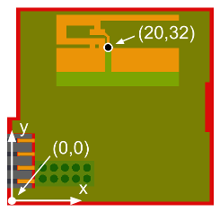
RFPort represents the input port of the antenna, thus has its Directionality attribute set to "in". RFModel stores the placement information about the antenna geometry, described in the linked Resource file, such as its X and Y position and rotation. The origin of the coordinate system is the top-side corner of the PCB closest to the EPM(s). The concept is illustrated below:

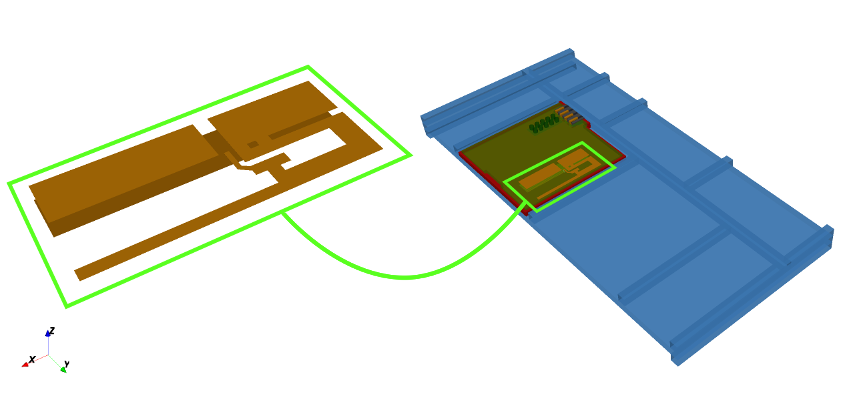
The Inverted-F antenna with ground planes "mounted" on a 2x2 Ara module.

Note that the antenna may be of arbitrary 3D shape and is not limited to PCB antennas.

InvertedFAssembly (Component Assembly)

The Component Assembly for the example model contains only the InvertedF antenna model connected to an RFPort with its Directionality attribute set to "in".

Excitation (Test Component)

This Test Component in the example design embodies the excitation for the Inverted-F antenna. It generates a 50 Ohm lumped-element resistor and the necessary voltage and current probes at the feed point, that is, between the bottom and the top of the PCB at the location defined in the attributes of the Inverted-F antenna model. During simulation it applies a 100~MHz bandwidth Gaussian excitation signal with the center frequency specified in the Frequency testbench parameter.

Usage

Performing an antenna analysis consists of the following simple steps. In the example model, steps 1-3 have already been done for you.

Make a copy of the desired testbench found under TestbenchLibrary / RF and adjust its name if necessary. In the example model, this has already been done: Directivity and SAR were copied to RFTest / InvertedF and renamed to InvertedFDirectivity and InvertedFSAR, respectively.
Create a reference to the component assembly to be tested, and connect it to the Excitation test component. In the example model, this has already been done using the InvertedF component assembly.
Configure the testbench parameters. See CyPhy2RF interpreter parameters for details. In the example model, this has already been done for you.
Make the testbench the active GME tab and invoke the master interpreter by clicking on its icon. See Using Test Benches for details on configuring and running Test Benches.
Find and inspect the produced analysis results in the folder indicated in the GME console. The results will be available once the analysis finishes running within the Job Manager.

Command-line Interface

An alternative approach to perform RF analysis is to use the AraRFAnalysis.exe command line tool. Assuming that the InvertedF.xml antenna description is found in the current directory, invoking the tool with the following parameters

"c:\Program Files (x86)\META\bin\AraRFAnalysis.exe" -x 20 -y 32 -r 0 --no-endo --module-size 2x2 InvertedF.xml

produces the same results as the execution of the above InvertedFDirectivity test bench. The mandatory parameters include the size of the Ara module (2x2), the path to the antenna model (InvertedF.xml) and its position (x = 20, y = 32) and rotation (r = 0°) in the module, relative to the top-side edge of the PCB closest to the EPM:

The above example also makes use of the --no-endo option, which reduces the simulation space to the size of the Ara module and speeds up the simulation for faster evaluation of the antenna parameters. For a detailed description of all the supported options please refer to the built-in help page of the tool by typing AraRFAnalysis.exe --help.

Interpretation of the results

The CyPhy toolsuite supports two RF analyses: Directivity and Specific Absorption Rate (SAR).

Directivity

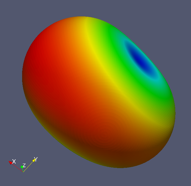
The directivity analysis focuses on the simulation of general antenna parameters, including the far-field directivity, S₁₁ and Z_IN at the given frequency. Currently, the analysis tool reports the maximum of the far-field pattern, a typical of which is shown in the figure below:

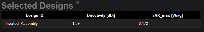
The typical far-field directivity of an antenna.

To view the results of the directivity analysis, open the Project Analyzer and navigate to the Design Space Analysis tab. If prompted, add all designs and variables. Then scroll to the Selected Designs section at the bottom to see results for Directivity in dBi.

SAR

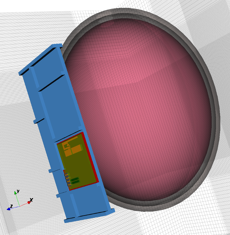
The goal of the Specific Absorption Rate (SAR) analysis is to estimate the rate at which the human body absorbs the energy radiated by the antenna. The CyPhy analysis tools intend to accurately reproduce the laboratory measurements defined by the FCC standard. That is, the simulation setup adds a phantom of the human head, see below, and estimates the SAR level averaged over volumes containing a mass of 1 gram of tissue.

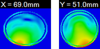
The simulation setup with a simple head phantom for SAR analysis.

The current SAR analysis calculates the SAR values over the entire head phantom, and reports is value along with cross-sections of the head at that location, see below.

The cross-sectional cuts of SAR values in the head phantom with plane normals X (left) and Y (right).

Note: That these values are not calibrated yet with actual laboratory measurements, and should be used only for comparative analysis for now.

To view the results of the SAR analysis, open the Project Analyzer and navigate to the Design Space Analysis tab. If prompted, add all designs and variables. Then scroll to the Selected Designs section at the bottom to see results for SAR_max in W/kg.

To view graphics depicting the amount of exposure at locations within the human head model, first right-click on the completed task in the Job Manager and select Show in Explorer. You may then view three image files depicting the intensity of the exposure: SAR-X.png, SAR-Y.png, and SAR-Z.png.