Using the PET Visualizer
Data from each PET run is stored in a .csv file in the generated execution
folder in the results directory;
however, OpenMETA has a built-in data visualizer for analysis and filtering.
1. Left-click Launch in OpenMETA Visualizer in the bottom-right corner of the Results Browser.
A browser window will open with the Visualizer.
- Navigate to the Pairs Plot tab of the Explore tab.
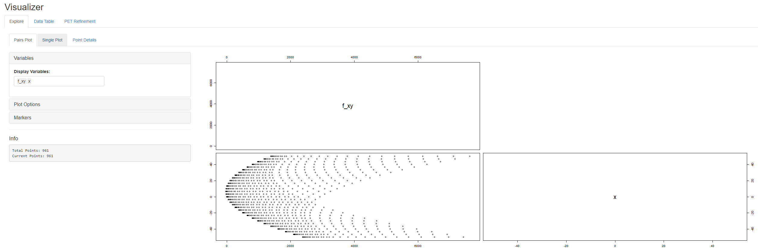
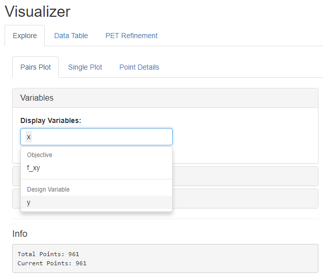
- Clear the default contents of the Display Variables field in the Variables section.
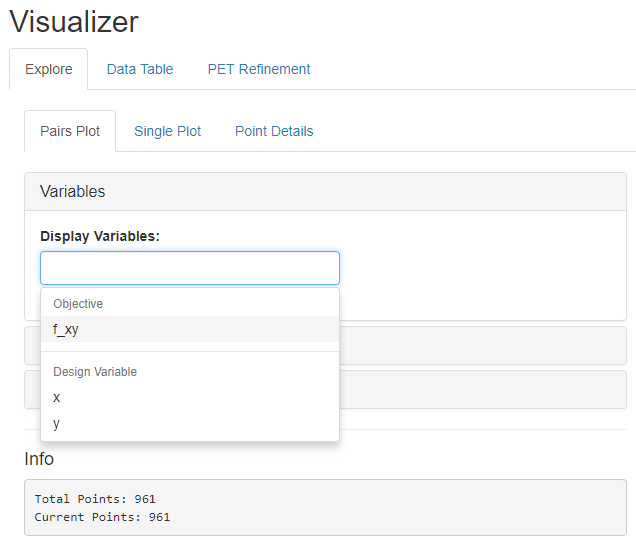
- Add x, y, and f_xy to the Display Variables field in that order.
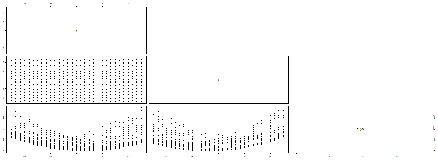
In the resulting matrix of scatter plots, each individual scatter plot displays the PET results across two different variables. The horizontal axis titles are at the top of each column, the vertical axis titles are to the right of each row, the vertical scale is on the left, and the horizontal scale is on the bottom. This technique allows all of the relationships between pairs of variables to be displayed on one screen.
The x vs. y plot clearly shows the full factorial distribution of the x and y Design Variable values.
The x vs. f_xy and y vs. f_xy plots suggest that f_xy’s minimum is found when both x and y are near the middle of their respective ranges.
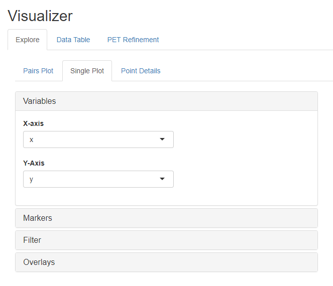
- Left-click the Single Plot tab of the Explore tab.
- Within the Variables section, left-click on the X-Axis menu and select x.
- Within the Variables section, left-click on the Y-Axis menu and select y.
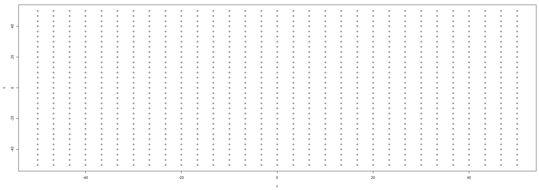
Since the x and y values were selected using a Full Factorial method, the resulting plot is not very interesting.
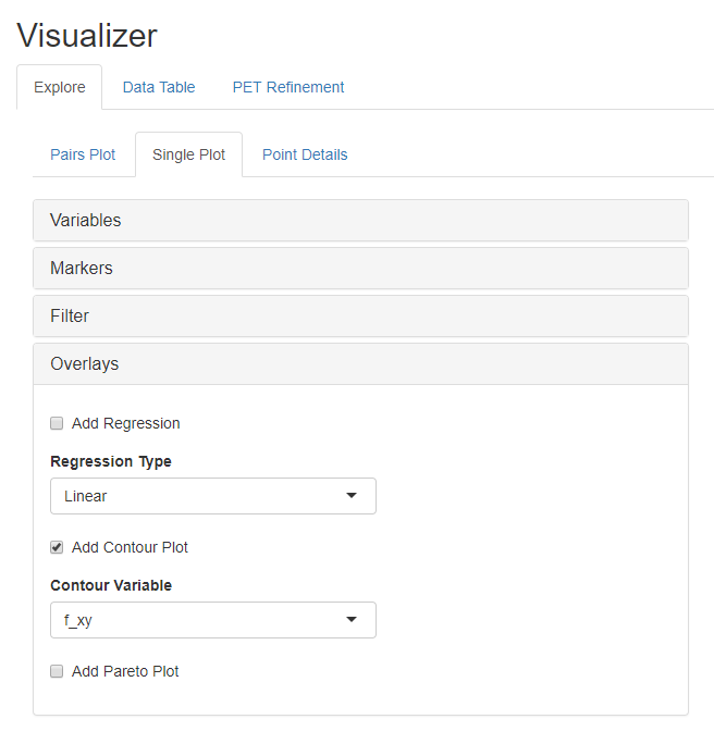
- Left-click on the Overlays section of Single Plot
- Select f_xy in the Contour Variable menu.
- Check the Add Contour Plot box
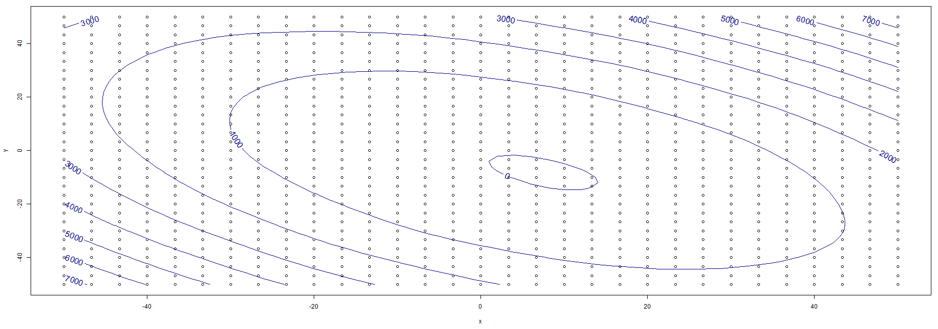
We have now added a contour plot overlay to our graph. The graphs shows us that f_xy appears to have a global minimum somewhere around (7,-8).
For more information on using the OpenMETA Visualizer, check out the Visualizer chapter.